Use Cases
Use Case 1: Plant-Wide Analysis of Control Loop Data
The Constraint Detection Add-on is suited for plant-wide analysis of control loop data. In this example, an asset tree with 111 controllers was analysed. Every controller has 4 signals assigned to it (Controller Output, Process Variable, Setpoint and Mode) which results in a total of 444 signals. The plant is divided into 2 sections where both sections have 6 units each. The structure of the asset tree and the number of controllers per unit is shown below.

Figure 1: Structure of the asset tree for use case 1
The asset tree was analysed over a period of one week and the Add-on looked for constraints/saturation in all controller outputs, process variables and setpoints. The copy of the asset tree was named “Plant Constraint Detection Results”. The thresholds were set to their default values 50% and 10%. No short capsules or gaps were specified.
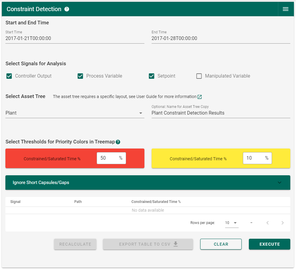
Figure 2: UI for use case 1
After the Add-on has finished the analysis, the table in the user interface is populated with the Top 30 of the most constrained/saturated signals in descending order. The table gives you a signal name and path, so that signals with a high ‘Constrained/Saturated Time %’ can be found easier in the treemap in the workbench. In addition, the table can be sorted by every column which gives you the option to target specific signal types or plant sections.
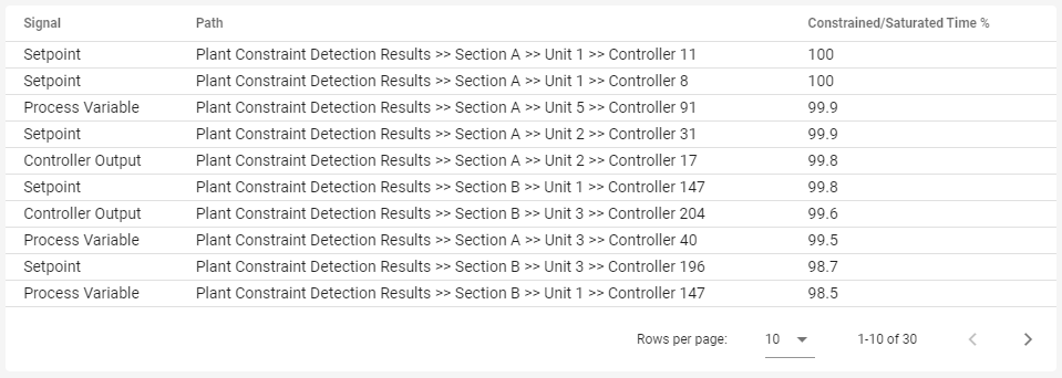
Figure 3: Index table for use case 1
The new “Plant Constraint Detection Results” asset tree can be found in the Data panel in the workbench. For every analysed signal, there are now 2 additional signals and 2 additional conditions:
Analysed Signal
Constraint/Saturation Signal
Constrained/Saturated Time Percentage
Medium Constraint/Saturation Condition
High Constraint/Saturation Condition
Based on the new signals and conditions, further analysis can be executed using the tools in the workbench.
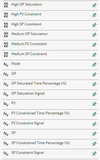
Figure 4: Signals and conditions in the “Plant Constraint Detection Results” asset tree for use case 1
In the workbench, three new worksheets called “OP Saturation Detection Treemap”, “PV Constraint Detection Treemap” and “SP Constraint Detection Treemap” have appeared. The treemap is coloured according to the thresholds which were set previously in the user interface. The ‘Constrained/Saturated Time %’ was selected as a statistic to be displayed in the treemap to facilitate the interpretation of the analysis results.
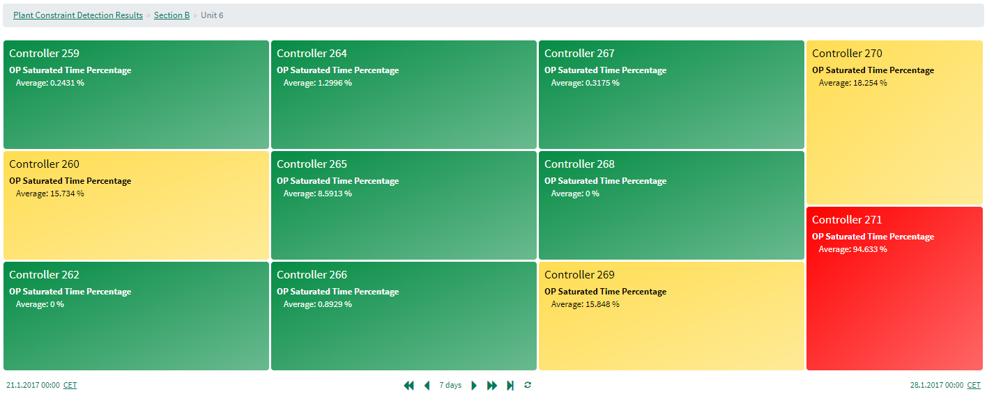
Figure 5: OP treemap for use case 1
From the treemap, it is easy to get to the trend view by clicking on a controller panel. In trend view, the constrained/saturated periods can be investigated in more detail and underlying causes for constraints/saturation can be identified.
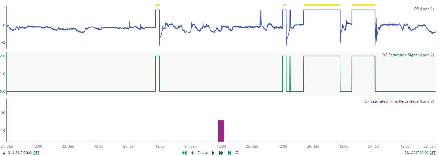
Figure 6: Trendview for use case 1
Use Case 2: Identifying Bad Actors
For the second use case, the asset tree from use case 1 was used again to identify bad actors. For this purpose, the thresholds for the treemap were adjusted. The red threshold and the yellow threshold were both set to 80%. Therefore, only red and green panels will appear in the treemap which makes it easier to find signals with a very a high ‘Constrained/Saturated Time %’. This use case shows how the threshold settings in the user interface can be used to get a treemap visualization which is tailored to the user’s requirements.
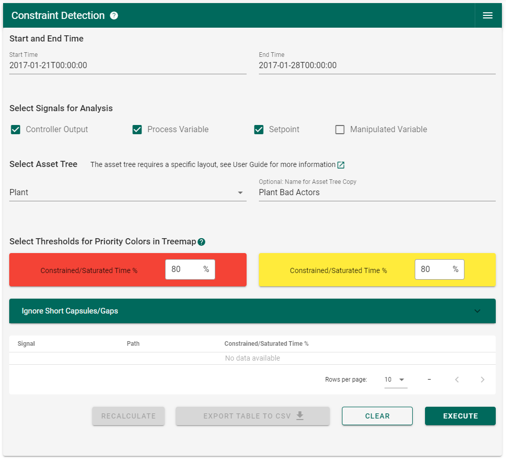
Figure 7: UI for use case 2
The analysis was performed over a period of one week and the new asset tree was named ‘Plant Bad Actors’. In the treemap, the controller outputs with a very high ‘Saturated Time %’ stand out and are easy to find, as can be seen below for controller 44 in Section A >> Unit 3.
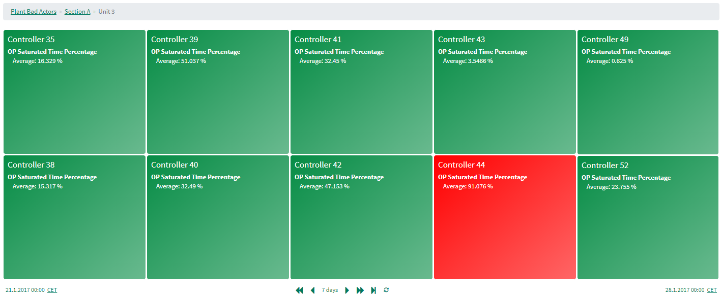
Figure 8: OP treemap for use case 2
If a bad actor is identified, the trend view for the corresponding controller can be investigated by clicking on the controller panel.
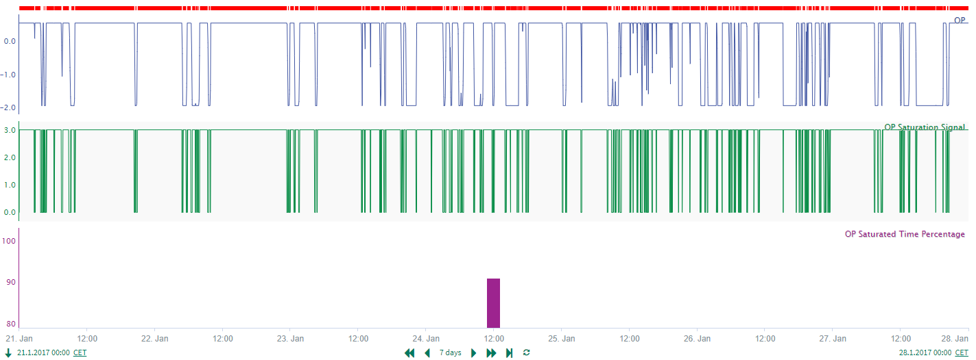
Figure 9: Trendview for use case 2
Note
Constraints and saturation in control signals are not always problematic because they can be an intended way of operation. For example, if controller output saturation is intended, then a signal with a high ‘Saturated Time %’ would not be a bad actor but a good actor. See Causes for Constraints and Saturation for more information.
Use Case 3: Setpoint Analysis for Constrained Model Predictive Control
In the third use case, the setpoints of the asset tree from use case 1 are examined. The setpoints are set by model predictive control (MPC). With MPC, a higher-level MPC controller calculates the setpoints of several lower-level controllers. The calculated setpoints can be constrained. This is called constrained MPC. In some cases, the constraints of the setpoints can be a process optimum. In this case, it is desired that a setpoint is at its constraint as often as possible in order to drive the process variable to the optimum (Use Case 3a). However, it may also not be desirable for a setpoint to always hit its constraint (Use Case 3b). For both cases, the Constraint Detection Add-on can be used.
In the first step, the ‘Plant’ asset tree was selected and the setpoint checkbox was activated so that a treemap for the setpoints is generated by the add-on. The new asset tree was named “Plant MPC Analysis”. The thresholds were set to 60% and 20%.
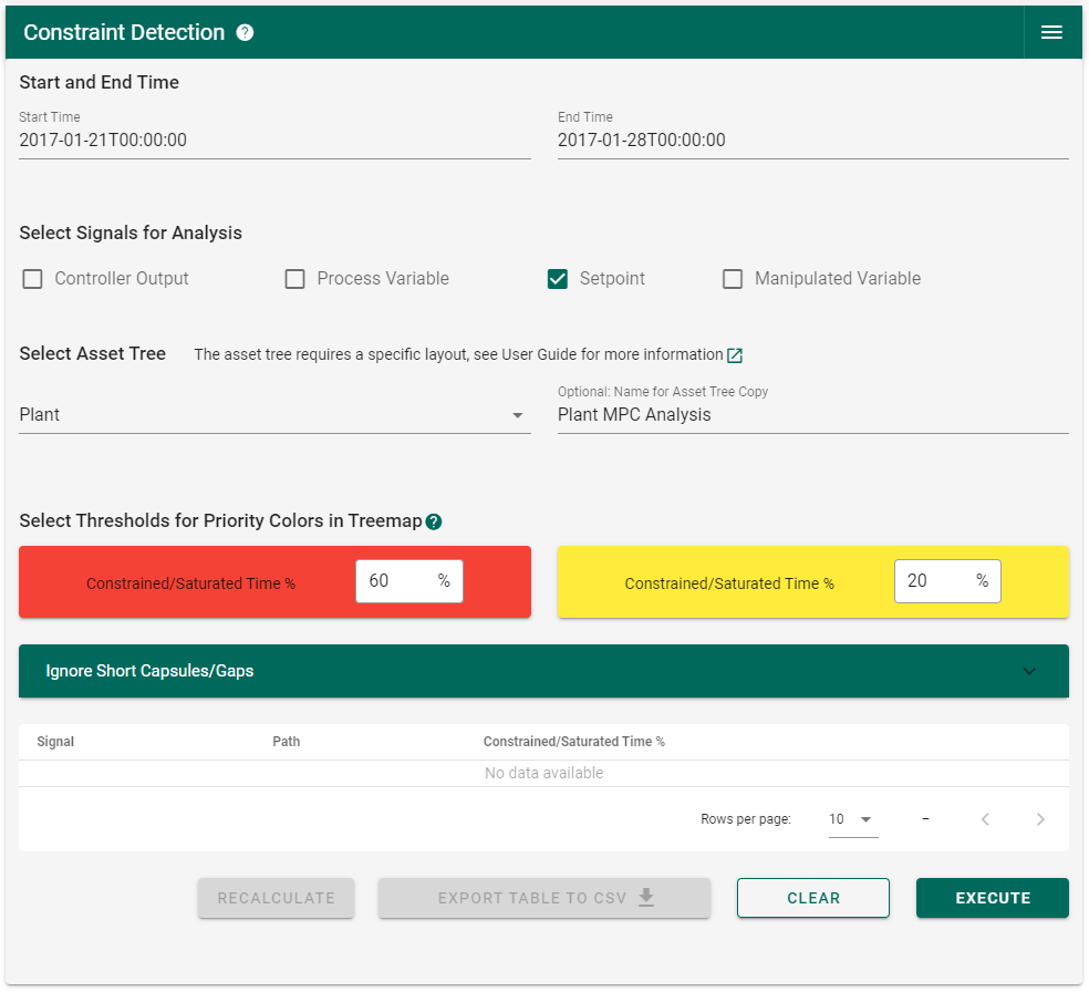
Figure 10: UI for use case 3
The Constraint Detection Add-on generated the treemap below for ‘Plant MPC Analysis >> Section A >> Unit 4’. There are two ways of interpreting this treemap depending on whether setpoint constraints are intentional or unintentional.
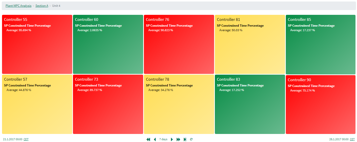
Figure 11: SP treemap for use case 3
Use Case 3a: Setpoint constraints are intentional
If setpoint constraints are intentional, setpoints with a high ‘Constrained Time %’ are good actors. That means that all red panels in the treemap show the intended way of operation. On the other hand, setpoints with a low ‘Constrained Time %’ will be shown as green panels in the treemap as they do not follow the intended way of operation. Consequently, the time trends of green panels can be investigated to determine why the setpoint is not driven to the optimum.
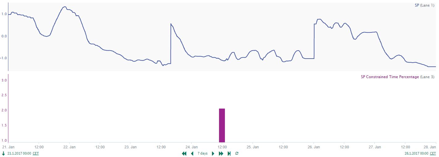
Figure 12: Trend view of the setpoint of controller 60 for use case 3
Use Case 3b: Setpoint constraints are unintentional
If setpoint constraints are unintentional, setpoints with a low ‘Constrained Time %’ are good actors. That means that all green panels in the treemap show the intended way of operation. On the other hand, setpoints with a high ‘Constrained Time %’ will be shown as red panels in the treemap as they do not follow the intended way of operation. Consequently, the time trends of red panels can be investigated to determine why the setpoint is reaching a constraint.
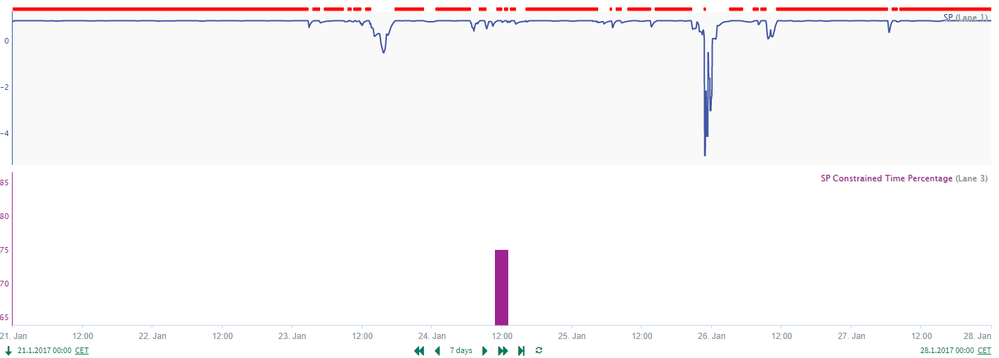
Figure 13: Trend view of the setpoint of controller 90 for use case 3
This use case illustrates how constraints can be both intentional and unintentional in control loops. Furthermore, it should be noted that even if constrained MPC is used, it is likely that there are both intentional setpoint constraints and unintentional setpoint constraints within the same plant. Therefore, each control loop should be considered individually.